

The Bitcoin Fear and Greed Index is certainly one of the most well-known sentiment indicators for Bitcoin, but is it really helpful when it comes to predicting future prices? Of course, one could easily create their own variants of a trend or sentiment indicator, but we want to test how well the “original” from alternative.me could be useful for predicting the bitcoin price.
The Bitcoin Fear and Greed Index, as it will turn out, seems to be surprisingly good at predicting the Bitcoin price. To that end, in this article we look at factor plots, the backtest of an exemplary strategy based on the index, and to visualize the effectiveness, the results of a linear strategy. However, the intransparent calculation of the index is problematic.
Bitcoin Fear and Greed Index: Correlation with the Bitcoin price?
It must be said at the outset that there are some limitations to consider here:
- The index is apparently closed source, so it is hard to tell how exactly the index values are composed.
- In addition, it is of course possible that the index was subsequently adjusted to the development of the Bitcoin price, i.e., after the prices were known (lookahead bias / backfitting).
- During its lifetime, the calculation of the index was changed. Originally, survey data was apparently included, but it is now no longer part of the index.
It is rarely a good idea to start an analysis without at least a vague hypothesis. So what would be a possible hypothesis here, especially since this is a sentiment index?
Be fearful when others are greedy, and greedy when others are fearful.
Warren Buffet
As a rule, one assumes that great euphoria occurs before a top and great despair before a low in stock prices. So we would expect, without having analyzed the data so far, that low values of the Fear and Greed Index would represent buying opportunities – conversely, values of the index in the “euphoria zone” would be potential sell signals. Do we find this pattern in the data?
Download data for the Bitcoin Fear and Greed Index
Fortunately, historical data for the Bitcoin Fear and Greed Index can be downloaded directly via an API.
The index fluctuates between values of 0 to 100, with minimum values of 5 and maximum values of 95 in the past history. The index starts at the beginning of 2018, so we have enough data to test the index in a meaningful way.
library(tidyverse)

dl <- read_lines("https://api.alternative.me/fng/?limit=2000&format=json&date_format=us")

library(rjson)
library(lubridate)

dl2 <- fromJSON(paste0(dl, collapse = " "))

dl2 <- map_dfr(dl2$data, function(x) {
    tibble(date = mdy(x$timestamp),
           value = as.numeric(x$value))
})

ggplot(dl2, aes(x = date, y = value)) +
    geom_point() +
    scale_y_continuous(breaks = scales::pretty_breaks(n = 20)) +
    geom_line() +
    theme_bw(base_size = 25) +
    ylab("") +
    xlab("") +
    ggtitle("Bitcoin Fear and Greed Index")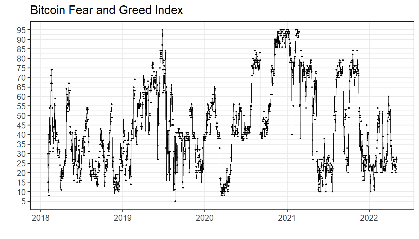
Download Bitcoin price data
Now, of course, we also need the Bitcoin price since 2018. Here, we use the tidyquant package for R to download this data from Tiingo. It is available after free registration if you want to reproduce this analysis. The API data is in JSON format, so it needs to be converted to a table format first before we can plot the data.
In this graph, we plotted the Bitcoin price since 2018 until April 2022 and colored each day according to the value of the Fear and Greed Index. You can see quite clearly that in the intermediate lows (crashes) of Bitcoin, the index values were low. In the substantial bull runs, on the other hand, the values were above 50 or even above 75, as in early 2021.
library(tidyquant)
tiingo_api_key('your_key')
btc <- tq_get(c("btcusd"),
       get = "tiingo.crypto",
       from = "2018-01-01"
       to = "2022-04-29",
       resample_frequency = "1day")

btc_plot <- left_join(
    btc,
    dl2
) %>%
    drop_na() %>%
    rename(`Fear and Greed Index` = value)

ggplot(btc_plot, aes(x = date, y = close, color = `Fear and Greed Index`)) +
    geom_line(size = 3) +
    geom_point(size = 3) +
    theme_classic(base_size = 25) +
    scale_y_log10(breaks = scales::pretty_breaks(n = 10)) +
    scale_color_viridis_c() +
ggtitle("Bitcoin 2018 - Today", "log scale") 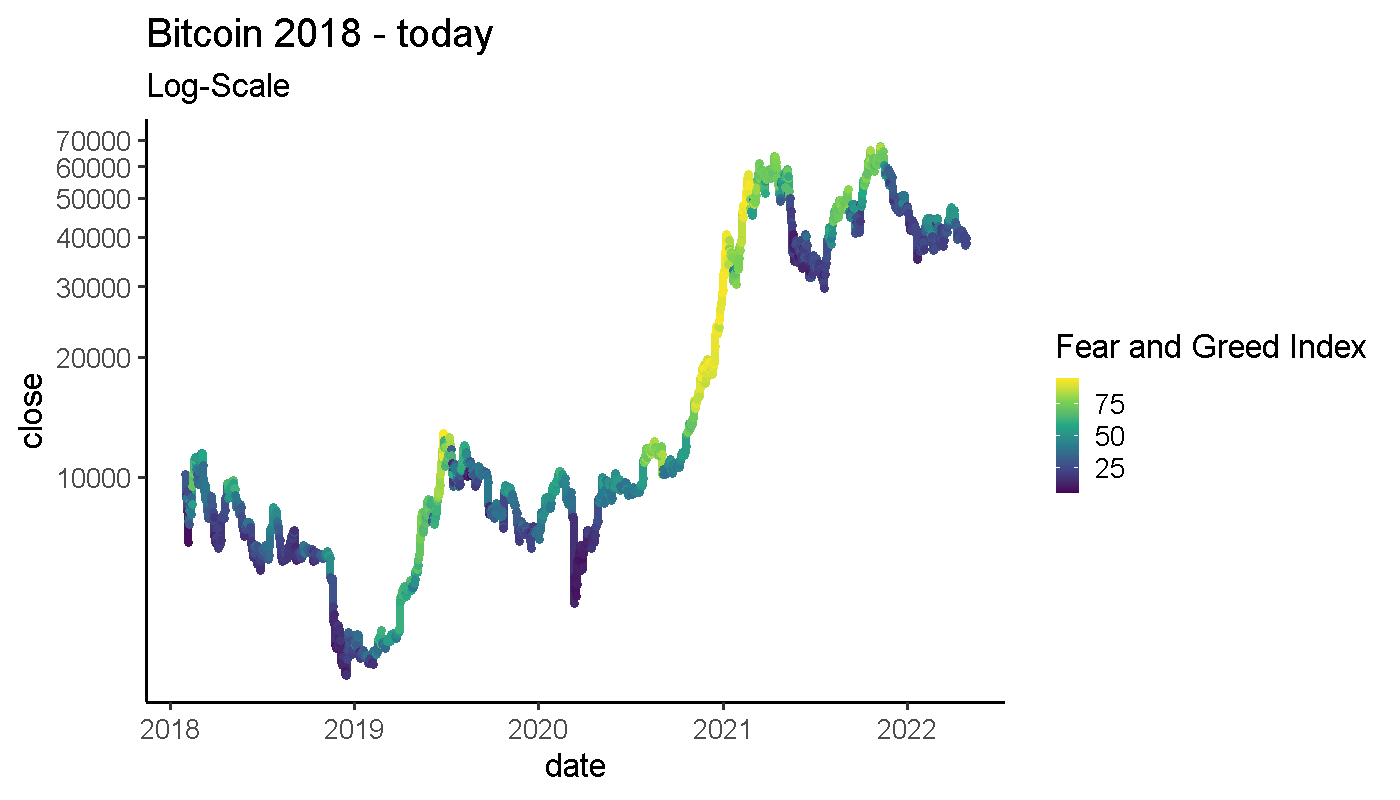
Bitcoin Fear and Greed Index analysis: data preparation
Now we create the lags (i.e. previous values) 1,5, …, 300 for the Fear and Greed Index. Then, in order to be able to examine the correlation between certain index values in the past with the Bitcoin price, we create similar lags of the Bitcoin price, but shifted one day into the future. Thus, we can relate yesterday’s index value to today’s bitcoin price, for example.
Of course, we would like to do the same not only for one day, but also for longer periods of time, hence the lags up to 300 days. For example, fg_300 is the value of the Fear and Greed Index 300 days ago and btc_return_300 is the bitcoin return in the 300 following days. This way we can always relate matching time periods.
dl2 <- dl2 %>%
    arrange(date) %>%
    mutate(
        fg_1 = dplyr::lag(value, 1),
        fg_5 = dplyr::lag(value, 5),
        fg_10 = dplyr::lag(value, 10),
        fg_20 = dplyr::lag(value, 20),
        fg_40 = dplyr::lag(value, 40),
        fg_300 = dplyr::lag(value, 300)
    ) %>%
    rename(fg = value)

btc2 <- btc %>%
    select(date, close) %>%
    mutate(date = as_date(date))

dat <- dl2 %>%
    left_join(btc2) %>%
    arrange(date) %>%
    mutate(
        btc_return_1 = lead(close) / close - 1,
        btc_return_5 = lead(close) / lag(close, 4) - 1,
        btc_return_10 = lead(close) / lag(close, 9) - 1,
        btc_return_20 = lead(close) / lag(close, 19) - 1,
        btc_return_40 = lead(close) / lag(close, 39) - 1,
        btc_return_300 = lead(close) / lag(close, 299) - 1
    )
Scatterplots of the Bitcoin Fear and Greed Index vs. Bitcoin Price
If for each day in the data we now plot the past value of the index with the corresponding Bitcoin return as a scatterplot, we get the following graphs. We simply used lag 20 here, but could have used 10 or 40 for example.
Surprisingly, we find a U-shape in most of the graphs. As mentioned at the beginning, we would rather have expected that low index values lead to high returns, while high index values lead to low returns. So more of a falling straight line. However, in the data we now see that apparently high index values also imply high Bitcoin returns. With index values around 50, the expected return is close to zero.
ggplot(dat %>%
         mutate(btc_return_20 = btc_return_20 * 100),
       aes(x = fg_20, y = btc_return_20)) +
    geom_point(size = 3, alpha = 0.3) +
    geom_smooth(size = 3, se = FALSE) +
    theme_classic() +
    xlim(0, 100) +
    xlab("Bitcoin Fear and Greed Index") +
    ylab("Bitcoin Return (%) 20 Days Later")
How stable is the relationship between the Bitcoin Fear and Greed and the price?
Another interesting plot is the binned barplot. Here we see the mean Bitcoin return depending on what range the index values were in. Again, we see the U-shape. For example, the expected return over the next 20 days when the Fear and Greed Index is between 10 and 20 is about 8%.
fg_20_bins <- dat %>%
    mutate(fg_20_bin = cut(x = fg_20, breaks = seq(from = 0, to = 100, by = 10))) %>%
    group_by(fg_20_bin) %>%
    summarise(mean_ret = mean(btc_return_20, na.rm = T)) %>%
    mutate(mean_ret = mean_ret * 100) %>%
    ungroup %>%
    drop_na()

ggplot(fg_20_bins, aes(x = fg_20_bin, y = mean_ret)) +
    geom_bar(stat = "identity") +
    xlab("Fear and Greed Index areas") +
    ylab("Mean BTC Yield (%)") +
    ggtitle("Relationship between BTC and areas of the Fear and Greed Index", "lag = 20") +
    theme_classic()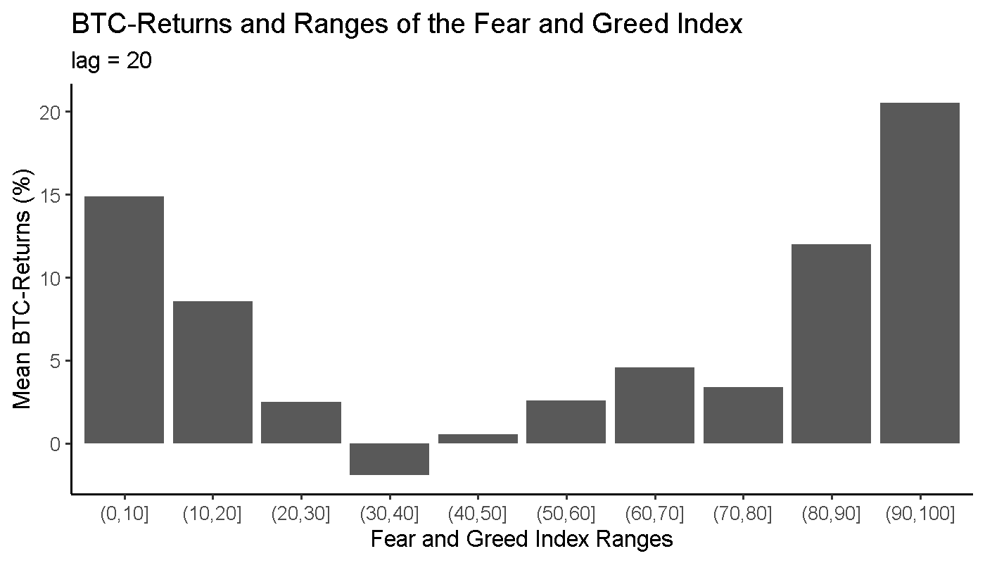
In addition, it is always interesting to see if these effects are stable over the years. Here, you will never find perfect stability, but in this case you can at least see the U-shape again quite well in most years. Some outliers could be due to the fact that in some years certain index values only occurred very rarely. For example, in 2019 there were only two days with index values above 90.
fg_20_bins <- date %>%
    mutate(year = year(date)) %>%
    mutate(fg_20_bin = cut(x = fg_20, breaks = seq(from = 0, to = 100, by = 10))) %>%
    group_by(fg_20_bin, year) %>%
    summarise(mean_ret = mean(btc_return_20, na.rm = T)) %>%
    mutate(mean_ret = mean_ret * 100) %>%
    ungroup %>%
    drop_na()

ggplot(fg_20_bins, aes(x = fg_20_bin, y = mean_ret)) +
    geom_bar(stat = "identity") +
    xlab("Fear and Greed Index areas") +
    ylab("Mean BTC Yield (%)") +
    ggtitle("Relationship between BTC and Fear and Greed Index ranges",
        "lag = 20") +
    theme_classic(base_size = 25) +
    theme(axis.text.x = element_text(angle = 90, vjust = 0.5, hjust=1)) +
    facet_wrap(~year)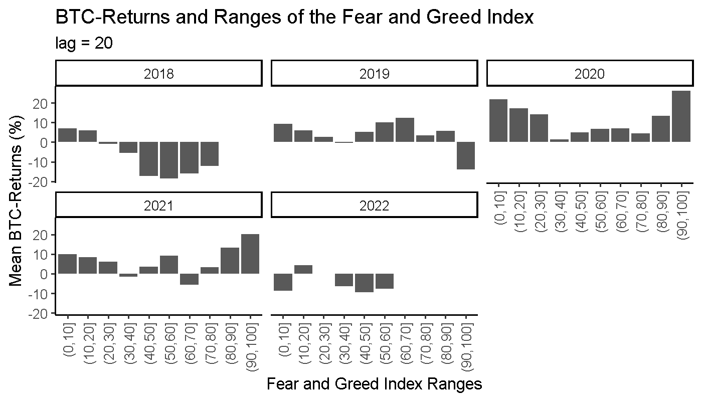
Backtest of the Bitcoin Fear and Greed Index
Linear Strategy
Before we move on to more realistic simulations, it is a good idea to backtest the presumed effect in as much isolation as possible. To do this, we build a linear strategy, where the Bitcoin exposure depends linearly (in the sense of a linear function) on the index values. The position size should be highest at the extreme values of the index, i.e., at 0 and 1, and it should be zero at index values of 50. After all, the U-shape in the relationship between index values and bitcoin returns that we found suggests that it would be beneficial to hold Bitcoin whenever the index is in the extreme ranges. So, in short, we use the following formula:
Size = abs(fear_and_greed – 50) / 50
Sizing the “linear” strategy
Thus, our position size automatically moves between 0 and 1. Zero would mean we hold 100% cash, and one would mean we hold 100% Bitcoin.
In this plot, we see by the coloring when we would now have high or low Bitcoin positions based on the linear strategy.
dat <- dat %>%
    ungroup() %>%
    mutate(lin_size = abs(fg_1 - 50) / 50)

ggplot(dat, aes(x = date, y = close, color = lin_size)) +
    geom_line(size = 3) +
    geom_point(size = 3) +
    scale_color_viridis_c() +
    theme_classic(base_size = 25) +
    xlab("") +
    ylab("Bitcoin") +
    ggtitle("Linear Strategy")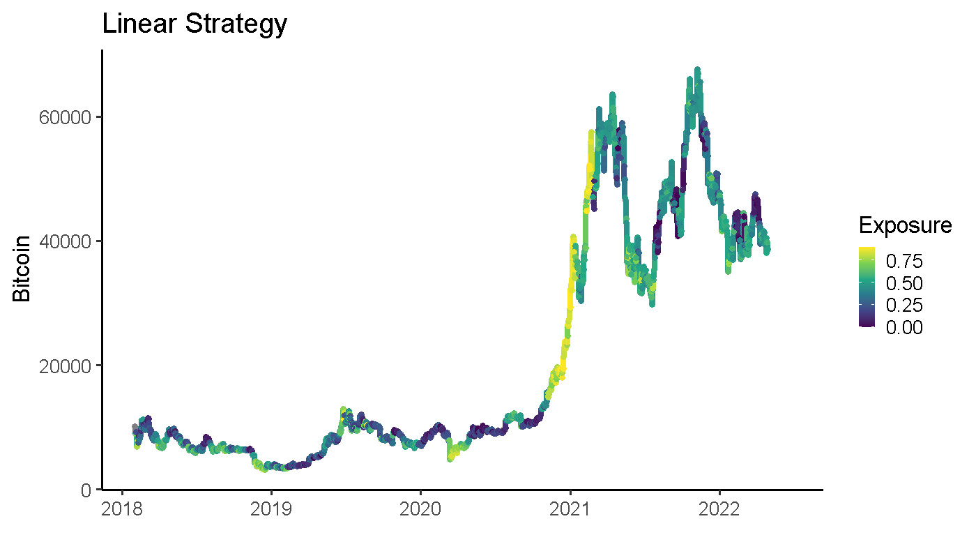
And this is what the capital growth would look like if this linear strategy was implemented. Transaction costs are not considered here, but again, the point is simply to look at the effect in isolation for now, before we start a more realistic test.
dat_bt <- dat %>%
    mutate(lin_strat_return = btc_return_1 * lin_size) %>%
    mutate(lin_strat_rev_return = btc_return_1 * (-lin_size + 1)) %>%
    select(date, close, lin_size, lin_strat_return, lin_strat_rev_return) %>%
    drop_na() %>%
    mutate(lin_strat_equity = cumprod(1 + lin_strat_return))

btc_ret <- btc %>%
    mutate(btc_ret = close / dplyr::lag(close) - 1) %>%
    select(date, btc_ret) %>%
    drop_na()
btc_ret_xts <- xts(btc_ret$btc_ret, order.by = btc_ret$date)
strat_ret_xts <- xts(dat_bt$lin_strat_return, order.by = dat_bt$date)
strat_ret_rev_xts <- xts(dat_bt$lin_strat_rev_return, order.by = dat_bt$date)
bt_xts <- merge(btc_ret_xts, strat_ret_xts, strat_ret_rev_xts)
bt_xts <- na.omit(bt_xts)
colnames(bt_xts) <- c("bitcoin", "linear strategy", "negative strategy")

charts.PerformanceSummary(bt_xts, geometric = F, main = "Linear Strategy")
# table.AnnualizedReturns(bt_xts, geometric = F, scale = 365)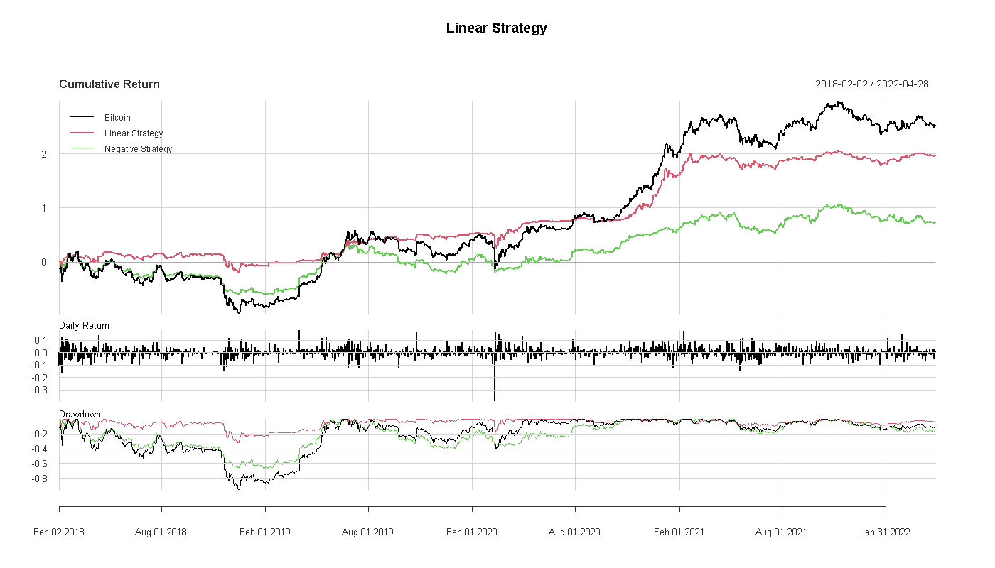
It is interesting to see that the linear strategy based on the Bitcoin Fear and Greed Index has lower returns than just holding Bitcoin, but has a much higher Sharpe ratio (1.18 instead of 0.8). Additionally, we have incorporated the negative of the linear strategy here, where the position size in Bitcoin would be maximal at intermediate index values. As expected, this strategy performs by far the worst.
Backtest with fixed cutoff for the BTC Fear and Greed Index
In practice, one would not follow the linear strategy where one would have to adjust the position size every day, but presumably one would choose one or more cutoffs above or below which one would then hold Bitcoin. Otherwise, one would stay in cash.
We’ll just take a cutoff of 15 and a 20 day holding period as an example here. So that means at index values below 15 or above (100 – 15) we buy Bitcoin and hold the position for 20 days.
With this cutoff and holding period, the strategy would have been completely in cash about two-thirds of the time, and in Bitcoin the rest of the time.
The results actually look quite appealing. Over the period since 2018, the strategy has achieved both higher returns and a much higher Sharpe ratio than just holding Bitcoin. Due to the small number of transactions, transaction costs should also not be a factor here, which is why we have not simulated these costs. The negative of the strategy is significantly worse than in the linear test and has a negative return.
dat <- dat %>%
dat_bt <- dat
dat_bt$signal <- NA

cutoff_long <- 15
cutoff_short <- 100 - 15
holding_period <- 20
for (i in 1:(nrow(dat_bt) - holding_period)) {
    if (dat_bt$fg[i] < cutoff_long | dat_bt$fg[i] > cutoff_short) {
        dat_bt$signal[(i+1):(i+holding_period)] <- 1
    }
}

dat_bt$signal[is.na(dat_bt$signal)] <- 0

dat_bt <- dat_bt %>%
    ungroup() %>%
    arrange(date) %>%
    mutate(fg_ret = ifelse(signal > 0.5, btc_return_1, 0)) %>%
    mutate(fg_ret_reverse = ifelse(signal < 0.5, btc_return_1, 0)) %>%
    select(date, fg_ret, fg_ret_reverse) %>%
    drop_na() %>%
    mutate(fg_equity = cumprod(1 + fg_ret))

btc_ret <- btc %>%
    mutate(btc_ret = close / dplyr::lag(close) - 1) %>%
    select(date, btc_ret) %>%
    drop_na()
btc_ret_xts <- xts(btc_ret$btc_ret, order.by = btc_ret$date)
strat_ret_xts <- xts(dat_bt$fg_ret, order.by = dat_bt$date)
strat_ret_rev_xts <- xts(dat_bt$fg_ret_reverse, order.by = dat_bt$date)
bt_xts <- merge(btc_ret_xts, strat_ret_xts, strat_ret_rev_xts)
bt_xts <- na.omit(bt_xts)

charts.PerformanceSummary(bt_xts, geometric = F)
| Bitcoin | Strategy | Negative Strategy | |
| Annualized Return | 42% | 49% | -7% |
| Annualized Std. Dev. | 0.63 | 0.40 | 0.48 |
| Annualized Sharpe Ratio | 0.67 | 1.24 | -0.15 |
Conclusion
So we have seen that the index seems to have been surprisingly useful in the past. At this point, we could still test whether the optimal cutoffs and holding period are stable over the years.
However, it would be more important to first take a step back here and consider what to do with these results in the first place.
The main problem remains that this is a proprietary index whose calculation is somewhat opaque. Moreover, our hypothesis that low values of the Fear and Greed Index lead to high Bitcoin returns, while high index values lead to low Bitcoin returns, has not been fully confirmed
Instead, high index values also led to high returns. Our guess is that this effect is an artifact of a momentum factor that may be included in the Fear and Greed Index. After all, the Bitcoin Fear and Greed Index is relatively close to classical factor analysis or some methods of so-called technical analysis.
So instead of adopting the original index unchanged now, one could create one’s own index based on such factors or (sentiment) indicators, which are a bit more transparent and comprehensible.
Moreover, mixing several factors in the Bitcoin Fear and Greed Index is somewhat problematic, as the performance of the individual factors cannot be viewed separately this way. Most recently, it appeared that the performance of the momentum factor in the crypto market, for example, was declining somewhat over the course of the last few years.
In summary, we were nevertheless surprised by how well the index would have performed if the values had indeed been arrived at without lookahead bias. An inquiry to alternative.me whether the index values were adjusted in the past and how they dealt with the removal of the survey data unfortunately remained unanswered.